winslow grid generation in curvilinear coordinates
Curvilinear coordinates allow finite-difference methods (FDM) to generlize to more complex geometries. The first step is to numerically evaluate a transform from the physical domain to the computational domain. While the geometry of physical domain can be quite complex, the computational domain is usually a rectangle:
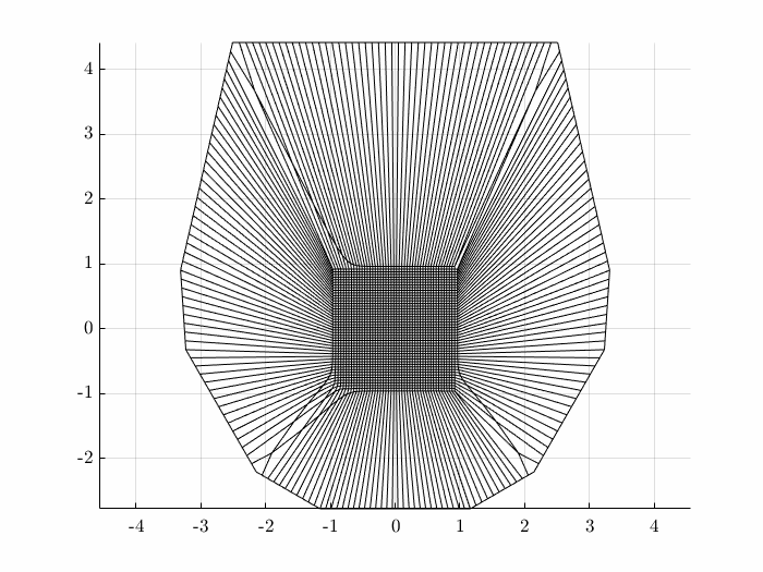
While there are many approaches to creating such a transform, one method is to solve the Winslow system of equations: \begin{equation} \alpha x_{\xi\xi} - 2\beta x_{\xi\eta} + \gamma x_{\eta\eta} = 0 \end{equation} \begin{equation} \alpha y_{\xi\xi} - 2\beta y_{\xi\eta} + \gamma y_{\eta\eta} = 0 \end{equation} with \begin{equation} \alpha = x_\eta^2 + y_\eta^2 \quad \gamma = x_\xi^2 + x_\xi^2 \quad \beta = x_\xi x_\eta + y_\xi y_\eta \end{equation} This coupled systems of equations may be solved iteratively to produce the desired grid: